| Category | Datasets |
|---|---|
| Market | Day-ahead prices; net positions |
| Load | Actual load; day-ahead load forecasts |
| Generation | Actual generation by technology; generation forecasts; wind and solar forecasts; intraday renewable forecasts; generation by plant |
| Capacity | Installed generation capacity; capacity by individual unit |
| Hydro | Aggregated hydro-reservoir and storage information |
| Balancing | Imbalance prices; imbalance volumes; activated balancing-energy prices |
| Outages | Generation-unit, production-unit and transmission unavailability |
| Transmission | Physical flows; total imports and exports; scheduled exchanges; day-ahead scheduled exchanges; intraday offered capacity; day-, week-, month- and year-ahead transfer capacity |
Day-Ahead Electricity Price Forecasting in the Baltic States
A short-window LEAR benchmark for Estonia, Latvia and Lithuania
Electricity markets
Forecasting
LASSO
Time series
A LASSO benchmark refitted every delivery day across 964 days of Baltic day-ahead prices — and what happens to it when the market turns violent.
Abstract
I build and evaluate day-ahead electricity price forecasts for the three Baltic bidding zones — Estonia, Latvia and Lithuania — using the LEAR (LASSO Estimated AutoRegressive) benchmark of Lago et al. (2021). The question is whether a parsimonious statistical model, given only local price history and the two day-ahead exogenous forecasts published before gate closure, produces useful forecasts across three small, tightly coupled markets, and how that performance holds up when prices turn violent.
A market database was assembled from the ENTSO-E Transparency Platform covering January 2015 to August 2026 — 29 distinct datasets across 150 dataset–area combinations — although the forecasting exercise deliberately draws on only three hourly series per zone. Each zone is modelled independently. Two rolling calibration windows are used, 8 weeks and 12 weeks, each refitted from scratch every delivery day, plus their arithmetic mean, referred to throughout as the short-window ensemble.
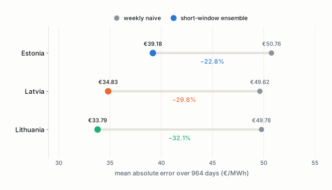
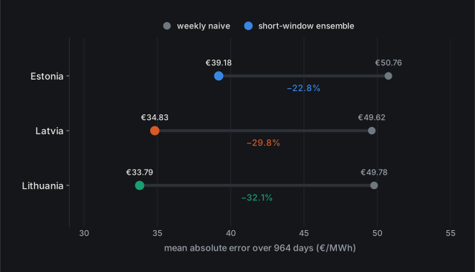
Over 964 out-of-sample delivery days — 23,136 hourly forecasts per model and zone — every LEAR specification beat a weekly naive forecast in every zone, and the ensemble was the strongest specification everywhere. Its rMAE was 0.772 in Estonia, 0.702 in Latvia and 0.679 in Lithuania: reductions in mean absolute error of roughly 23%, 30% and 32% against using last week’s price at the same hour.
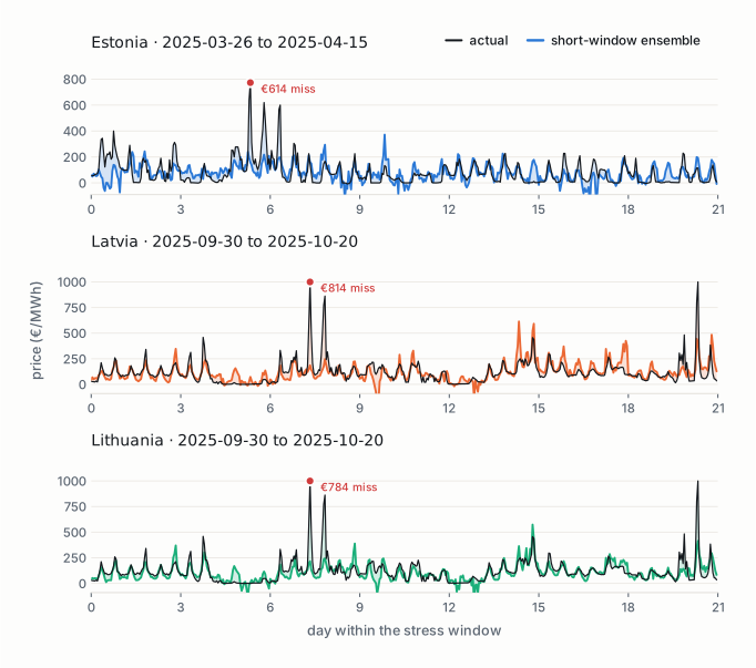
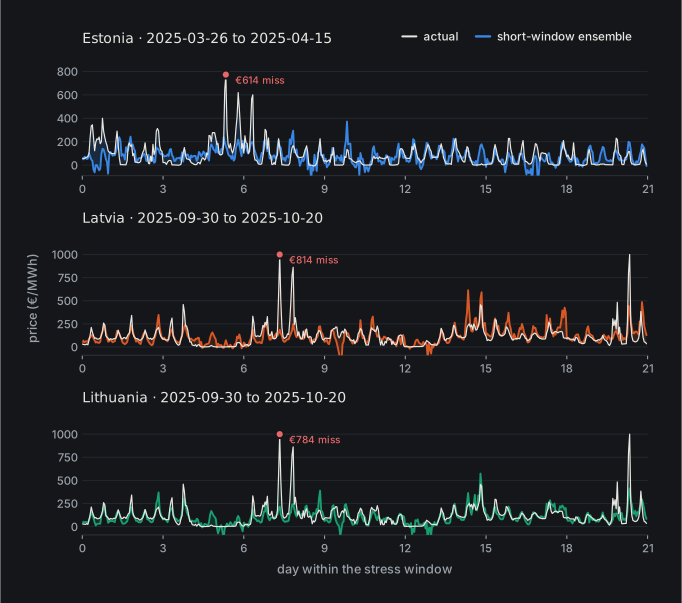
That average conceals the model’s real weakness. Inside each zone’s most volatile 21-day stretch, ensemble rMAE rose to 0.855, 0.905 and 0.826, and single hourly errors exceeded €600/MWh in Estonia and €780–815/MWh in Latvia and Lithuania. The ensemble still beat the naive benchmark under stress — in Latvia by only 9.5%, against 29.8% over the full sample. A model can be good on average and still miss precisely the hours that carry the commercial risk.
Keywords — electricity price forecasting; LEAR; LASSO; ENTSO-E; Baltic electricity market; rolling recalibration; forecast combination; price volatility.
1. Data
1.1 Collection
The dataset was pulled directly from the ENTSO-E Transparency Platform through its API, using Python and the entsoe-py interface. A dedicated downloader walked the archive month by month from January 2015. Monthly granularity was chosen deliberately: it makes the download resumable, and it stops a single API failure from corrupting or interrupting the full historical pull.
Original ENTSO-E observations are stored separately by dataset, area and month in compressed CSV, preserving a raw layer beneath every later transformation. Requests that returned nothing were logged as empty rather than backfilled with artificial observations — an important distinction, because a silently interpolated gap is indistinguishable from data once it reaches a model. The resulting inventory holds 150 dataset–area combinations drawn from 29 dataset types across eight categories.
The downloader also collected bilateral data for the main Baltic interconnections — Estonia–Latvia, Estonia–Finland, Latvia–Lithuania, Lithuania–Sweden (SE4) and Lithuania–Poland — querying both directions of every border. None of it enters the model below. It exists because the interesting version of this project is the one that uses it.
Coverage is uneven, as it always is: not every ENTSO-E endpoint is populated for every country and period. Prices, load, generation and generation forecasts are close to complete across 2015–2026. Balancing, outage and some transfer-capacity series are considerably more fragmented.
1.2 What the model is actually given
Although the archive is broad, the LEAR exercise uses a deliberately restricted information set, to stay close to the Nord Pool benchmark design in Lago et al. That benchmark pairs hourly day-ahead prices with a day-ahead load forecast and a day-ahead wind-generation forecast. For each zone:
- \(p_{d,h}\) — the day-ahead price for delivery day \(d\), hour \(h\) (the target);
- \(x^{1}_{d,h}\) — the day-ahead load forecast;
- \(x^{2}_{d,h}\) — the day-ahead wind-generation forecast.
Both exogenous series are published before the day-ahead auction closes, so they are legitimately available when the forecast for day \(d\) has to be made. No realized load, realized generation or realized physical flow appears anywhere in the model. Estonia, Latvia and Lithuania are modelled independently: the Estonian model forecasts Estonian prices from Estonian predictors, and so on.
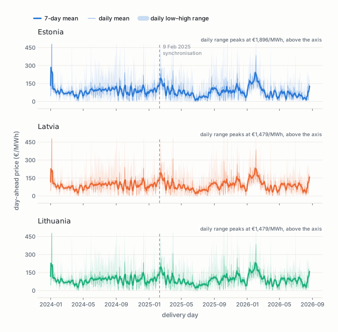
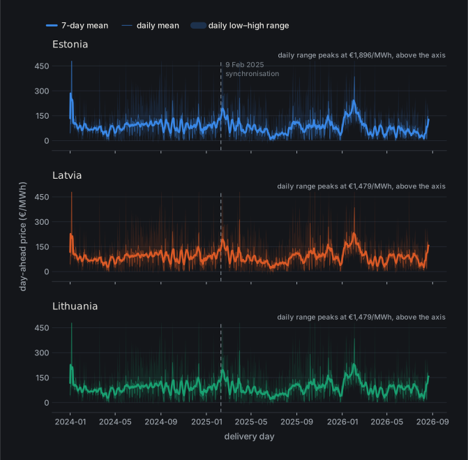
Figure 1 is the series being forecast. Three things in it matter for everything that follows. Prices are spiky rather than merely variable — the daily high runs to €1,896/MWh in Estonia. The three zones move together closely enough that Latvia and Lithuania are frequently the same number. And the character of the series changes over the sample: the calm middle of 2025 and the turbulent turn of 2026 are different forecasting problems.
1.3 Preparation
ENTSO-E series arrive at different temporal resolutions, so everything was converted to a consistent hourly structure. Daylight-saving transitions were handled by averaging the duplicated autumn hour and interpolating the missing spring hour, following the convention used for the benchmark datasets in Lago et al.
Missing observations were treated conservatively. Short internal gaps were interpolated where the regular hourly structure epftoolbox requires demanded it. Estonia’s evaluation period contained one isolated full-day gap in the wind forecast, reconstructed from the average of the same hour on the immediately preceding and following complete days. Larger historical gaps falling outside any rolling calibration window were left untouched. All of this was done on derived modelling files; the downloaded raw layer was never edited.
2. Methodology
2.1 The forecasting problem
The object to forecast is the full vector of 24 day-ahead prices,
\[ \mathbf{p}_d = [\,p_{d,1},\, p_{d,2},\, \ldots,\, p_{d,24}\,]^{\top}, \]
with all 24 values committed at once, before gate closure. In a linear framework the price for delivery hour \(h\) is
\[ p_{d,h} = \boldsymbol{\theta}_h^{\top}\mathbf{X}_{d,h} + \varepsilon_{d,h}, \]
where \(\mathbf{X}_{d,h}\) holds the predictors available before delivery, \(\boldsymbol{\theta}_h\) the coefficients for hour \(h\), and \(\varepsilon_{d,h}\) the forecast error. Each of the 24 hours gets its own equation.
2.2 The LEAR specification
LEAR is a parameter-rich autoregressive model with exogenous variables. Rather than pre-selecting a small set of regressors, it is handed a large candidate set and lets \(L_1\) regularisation decide what survives.
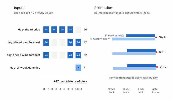
For delivery day \(d\) the information set contains four historical price vectors (\(\mathbf{p}_{d-1}\), \(\mathbf{p}_{d-2}\), \(\mathbf{p}_{d-3}\), \(\mathbf{p}_{d-7}\)), the two day-ahead exogenous forecasts for the delivery day itself (\(\mathbf{x}^1_d\), \(\mathbf{x}^2_d\)), their values one day and one week earlier (\(\mathbf{x}^1_{d-1}\), \(\mathbf{x}^1_{d-7}\), \(\mathbf{x}^2_{d-1}\), \(\mathbf{x}^2_{d-7}\)), and seven day-of-week dummies. Written out for hour \(h\):
\[ \begin{aligned} p_{d,h} =\;& \sum_{i=1}^{24}\theta_{h,i}\,p_{d-1,i} + \sum_{i=1}^{24}\theta_{h,24+i}\,p_{d-2,i} + \sum_{i=1}^{24}\theta_{h,48+i}\,p_{d-3,i} + \sum_{i=1}^{24}\theta_{h,72+i}\,p_{d-7,i} \\[2pt] &+ \sum_{i=1}^{24}\theta_{h,96+i}\,x^{1}_{d,i} + \sum_{i=1}^{24}\theta_{h,120+i}\,x^{2}_{d,i} \\[2pt] &+ \sum_{i=1}^{24}\theta_{h,144+i}\,x^{1}_{d-1,i} + \sum_{i=1}^{24}\theta_{h,168+i}\,x^{2}_{d-1,i} \\[2pt] &+ \sum_{i=1}^{24}\theta_{h,192+i}\,x^{1}_{d-7,i} + \sum_{i=1}^{24}\theta_{h,216+i}\,x^{2}_{d-7,i} + \sum_{i=1}^{7}\theta_{h,240+i}\,z_{d,i} + \varepsilon_{d,h}. \end{aligned} \]
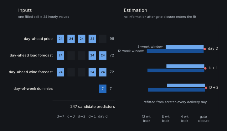
That is 247 candidate predictors per hourly equation: 96 price lags, 72 load-forecast terms, 72 wind-forecast terms and seven day-of-week indicators (Figure 2, left). The dimension is the point — it is high enough that regularisation has to do real feature selection.
2.3 Estimation
The coefficients are estimated by the LASSO objective
\[ \hat{\boldsymbol{\theta}}_h = \underset{\boldsymbol{\theta}_h}{\arg\min} \left[\, \mathrm{RSS} \;+\; \lambda \sum_{j=1}^{247}\lvert\theta_{h,j}\rvert \,\right], \]
where \(\mathrm{RSS}\) is the residual sum of squares and \(\lambda\) sets the strength of the penalty. The \(L_1\) penalty drives coefficients exactly to zero, so estimation and feature selection happen in one step: predictors that add nothing are removed from the equation rather than shrunk toward irrelevance.
Following the epftoolbox implementation, \(\lambda\) is chosen along the LARS path by the Akaike Information Criterion, after which the model is re-estimated by ordinary coordinate-descent LASSO. This is the computationally cheap procedure proposed in the benchmark study, and it is what makes daily recalibration affordable at all.
2.4 Variance stabilisation
Electricity prices are badly non-Gaussian: heavy right tails, and genuine negative values. A log transformation is therefore unavailable. LEAR instead uses the inverse hyperbolic sine,
\[ \operatorname{asinh}(x) = \ln\!\left(x + \sqrt{x^{2}+1}\right), \]
applied after robust centring and scaling. It behaves approximately linearly near zero and logarithmically in both tails, so it compresses extreme observations without ever becoming undefined for zero or negative prices.
2.5 Calibration windows and daily recalibration
A calibration window is how much history is used to fit the model for one particular forecast day; the following day, the model is refitted on a window shifted forward by one. Lago et al. insist on daily recalibration because a model estimated once and left alone does not describe how electricity price forecasting actually works.
The original benchmark evaluates four windows — 8 weeks, 12 weeks, three years and four years. Computational cost forced a narrower choice here:
\[ W_1 = 56 \text{ days}, \qquad W_2 = 84 \text{ days}. \]
A separate model is re-estimated every day for each window, and the short-window ensemble is their arithmetic mean,
\[ \hat p^{\,\mathrm{ENS}}_{d,h} = \tfrac{1}{2}\left(\hat p^{\,8\mathrm{w}}_{d,h} + \hat p^{\,12\mathrm{w}}_{d,h}\right). \]
This is an adaptation of the forecast-combination principle in Lago et al., not their four-window ensemble, and it is named accordingly throughout.
2.6 Out-of-sample design
The test period runs from 1 January 2024 to 21 August 2026: 964 forecast days, 23,136 hourly forecasts per model and zone. It is the final segment of the available data rather than a random sample, so no test observation is ever available to a model that is forecasting an earlier day.
For exploratory purposes, results are additionally split around 9 February 2025, when the three Baltic systems desynchronised from the Russian and Belarusian grids and joined the Continental European Synchronous Area. The split is descriptive. It is not, and is not treated as, evidence that synchronisation caused anything.
2.7 Evaluation metrics
Three point-forecast metrics are reported. Mean absolute error,
\[ \mathrm{MAE} = \frac{1}{24 N_d}\sum_{d=1}^{N_d}\sum_{h=1}^{24} \bigl\lvert p_{d,h} - \hat p_{d,h} \bigr\rvert , \]
root mean squared error, which punishes large misses far harder,
\[ \mathrm{RMSE} = \sqrt{\frac{1}{24 N_d}\sum_{d=1}^{N_d}\sum_{h=1}^{24} \bigl(p_{d,h} - \hat p_{d,h}\bigr)^{2}} , \]
and the relative measure that carries most of the argument below,
\[ \mathrm{rMAE} = \frac{\sum_{d,h}\lvert p_{d,h} - \hat p_{d,h}\rvert} {\sum_{d,h}\lvert p_{d,h} - \hat p^{\,\mathrm{naive}}_{d,h}\rvert}, \qquad \hat p^{\,\mathrm{naive}}_{d,h} = p_{d-7,h}. \]
The naive forecast is last week’s price at the same hour — a benchmark that is harder to beat than it sounds, because it preserves both the daily and the weekly shape of the price curve for free. An rMAE below 1 means the model beats it. Lago et al. prefer this measure because it is comparable across markets of different price levels, which is exactly the comparison being made here.
3. Results
3.1 Full-sample accuracy
Every specification beats the weekly naive benchmark in every zone, and the ensemble is the strongest specification everywhere, on all three metrics.
| Zone | Model | MAE (€/MWh) | RMSE (€/MWh) | rMAE | MAE vs naive |
|---|---|---|---|---|---|
| Estonia | LEAR 8w | 40.72 | 68.87 | 0.802 | −19.8% |
| Estonia | LEAR 12w | 41.46 | 70.62 | 0.817 | −18.3% |
| Estonia | Ensemble | 39.18 | 65.52 | 0.772 | −22.8% |
| Latvia | LEAR 8w | 36.41 | 58.92 | 0.734 | −26.6% |
| Latvia | LEAR 12w | 36.60 | 58.79 | 0.738 | −26.2% |
| Latvia | Ensemble | 34.83 | 56.23 | 0.702 | −29.8% |
| Lithuania | LEAR 8w | 35.24 | 57.20 | 0.708 | −29.2% |
| Lithuania | LEAR 12w | 35.43 | 57.97 | 0.712 | −28.8% |
| Lithuania | Ensemble | 33.79 | 55.27 | 0.679 | −32.1% |
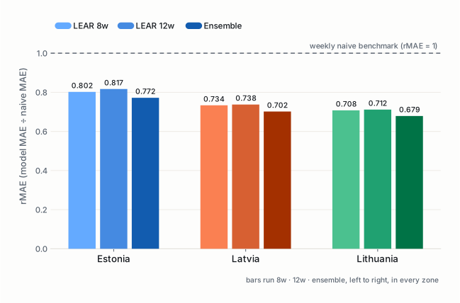
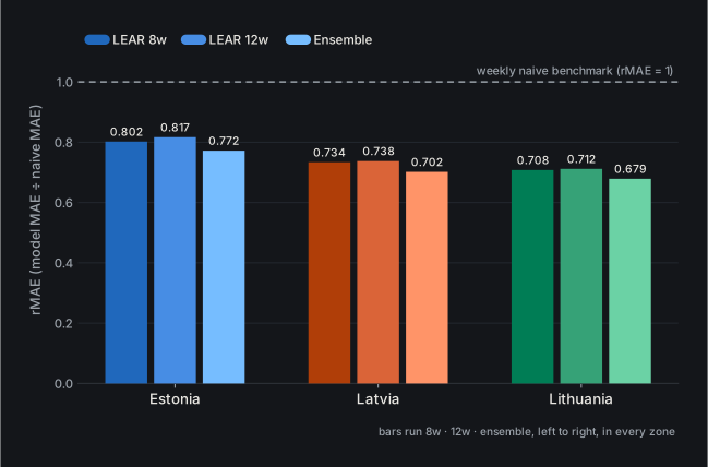
Lithuania is the easiest of the three markets for this information set, followed by Latvia; Estonia is the hardest. The ensemble cuts mean absolute error by 22.8% in Estonia, 29.8% in Latvia and 32.1% in Lithuania (Figure 4).
The 8-week specification edges out the 12-week one over the complete sample in all three zones, but the gaps are small — 0.015, 0.004 and 0.004 in rMAE — and without a Diebold–Mariano or Giacomini–White test there is no basis for calling any of them real. That test is the most obvious thing missing from this analysis and is listed as such in §5.
3.2 Accuracy over time
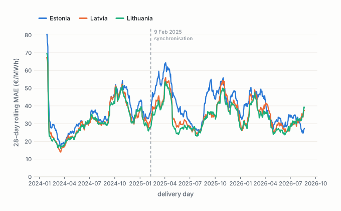
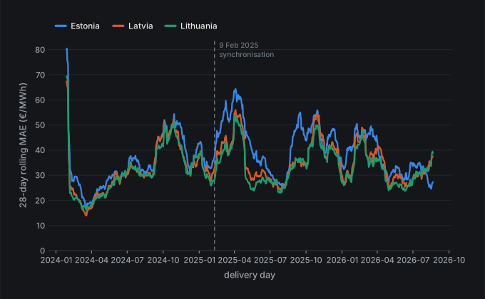
The aggregate table hides how unevenly that accuracy is distributed. Figure 5 tracks a 28-day rolling MAE across the whole evaluation period. The three zones move almost in lockstep — unsurprising, given how tightly coupled they are — and the level wanders between roughly €20/MWh in the calm middle of 2024 and €60/MWh in the spring of 2025 and again in early 2026. A single full-sample MAE is an average over regimes that differ by a factor of three.
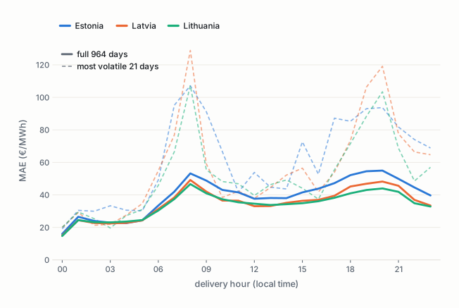
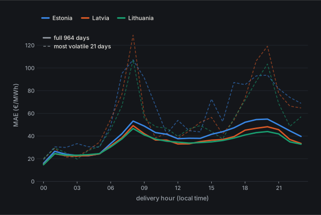
The daily profile is just as uneven (Figure 6). Error concentrates in the morning ramp around 08:00 and the evening peak around 19:00–20:00, and collapses overnight. The hours that are hardest to forecast are the hours in which the most money changes hands.
3.3 The shape of the errors
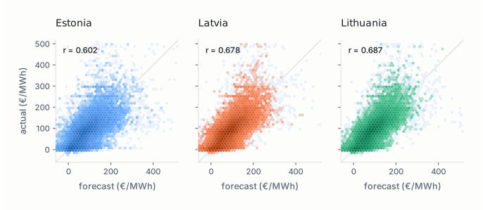
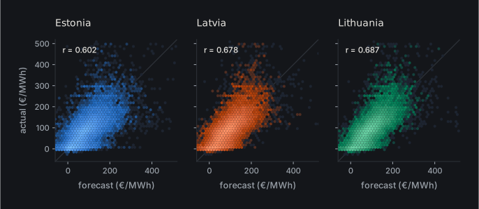
Figure 7 plots every hourly forecast against what actually cleared. The bulk of the mass sits along the diagonal, which is what a working forecast looks like. The interesting part is the vertical smear above it: hours where the market cleared far higher than the model expected. There is no comparable smear below the diagonal. The model rarely invents a spike; it routinely fails to anticipate one.
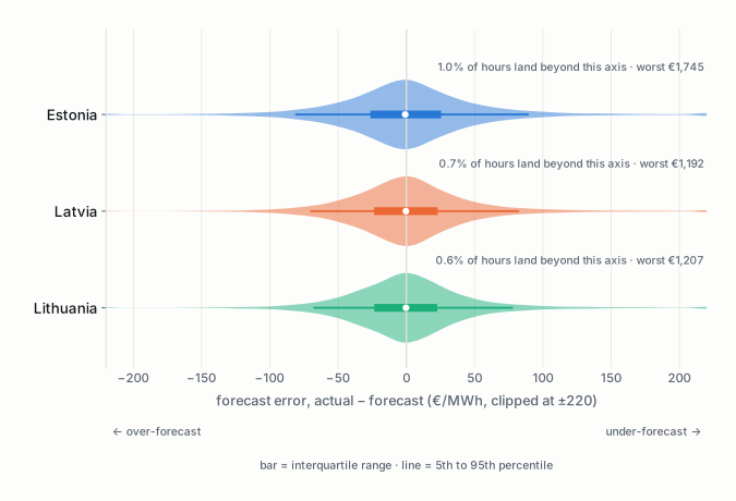
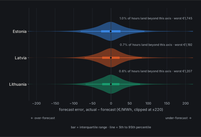
The error distribution says the same thing more precisely (Figure 8). The centre is tight — the interquartile range is comfortably inside ±€30/MWh in all three zones, and the median error is within €1/MWh of zero — but 0.6% to 1.0% of hours land beyond ±€220/MWh, and the single worst hour of the sample reaches €1,745/MWh in Estonia. This is the distribution that produces an RMSE of €65/MWh from an MAE of €39/MWh.
3.4 Around the February 2025 synchronisation
The three metrics disagree about what happened after 9 February 2025, and the disagreement is the interesting part (Figure 9).
| Zone | Days before / after | MAE before → after | RMSE before → after | rMAE before → after |
|---|---|---|---|---|
| Estonia | 405 / 559 | €37.37 → €40.50 | €71.52 → €60.81 | 0.780 → 0.773 |
| Latvia | 405 / 559 | €33.74 → €35.62 | €59.41 → €53.80 | 0.712 → 0.701 |
| Lithuania | 405 / 559 | €33.38 → €34.10 | €61.31 → €50.45 | 0.703 → 0.668 |
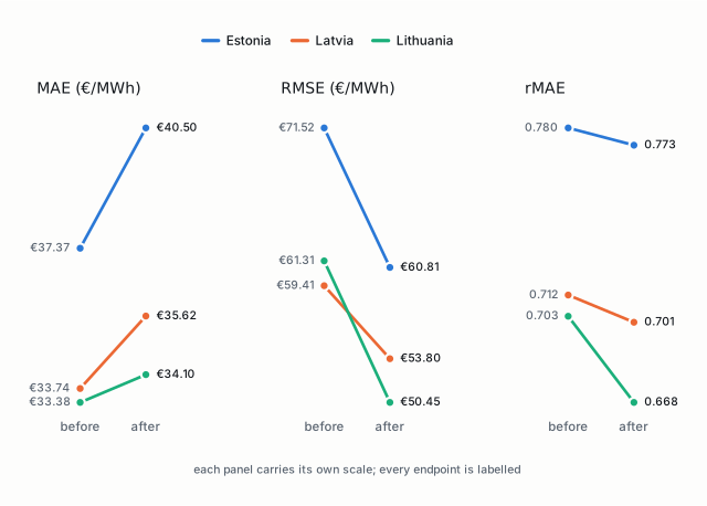
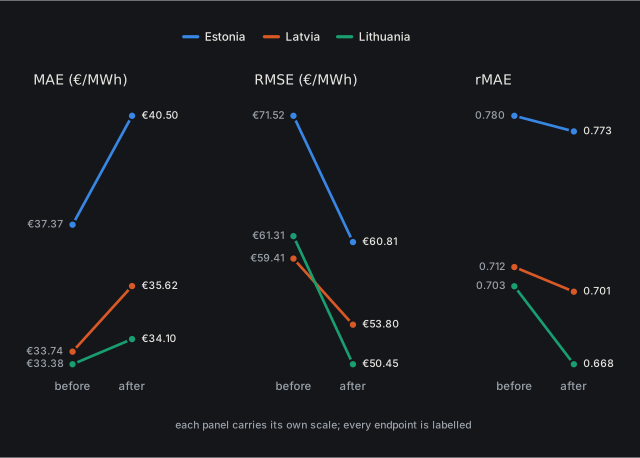
Relative performance does not deteriorate after synchronisation — it improves slightly in Estonia and Latvia and visibly in Lithuania, from 0.703 to 0.668. Absolute MAE rises modestly everywhere. But RMSE falls, and falls hard: from €71.52 to €60.81/MWh in Estonia, €59.41 to €53.80 in Latvia, €61.31 to €50.45 in Lithuania.
One reading is that typical errors grew slightly while the largest errors became rarer or smaller. That is consistent with all three metrics, but it is inferred from aggregates, and it should be checked directly against the error distributions before anyone believes it. More importantly, none of this identifies an effect of synchronisation. A credible causal design would need formal change-point tests and controls for everything else that moved at the same time — fuel prices, renewable output, transmission conditions, demand and market coupling. What the table shows is that the model did not break.
4. Under stress
Aggregate accuracy hides the model’s behaviour in exactly the conditions that matter most commercially. So each zone was evaluated again inside its own worst window: the 21-day interval with the highest rolling average of within-day price standard deviation.
| Zone | Model | MAE (€/MWh) | RMSE (€/MWh) | rMAE | rMAE, full sample | Worst hour (€/MWh) |
|---|---|---|---|---|---|---|
| Estonia | LEAR 8w | 65.66 | 97.34 | 0.913 | 0.802 | 625 |
| Estonia | LEAR 12w | 63.84 | 93.02 | 0.888 | 0.817 | 603 |
| Estonia | Ensemble | 61.50 | 90.73 | 0.855 | 0.772 | 614 |
| Latvia | LEAR 8w | 58.12 | 103.04 | 0.935 | 0.734 | 814 |
| Latvia | LEAR 12w | 58.15 | 100.55 | 0.936 | 0.738 | 815 |
| Latvia | Ensemble | 56.21 | 99.29 | 0.905 | 0.702 | 814 |
| Lithuania | LEAR 8w | 54.73 | 94.35 | 0.881 | 0.708 | 809 |
| Lithuania | LEAR 12w | 52.53 | 92.14 | 0.845 | 0.712 | 760 |
| Lithuania | Ensemble | 51.35 | 90.60 | 0.826 | 0.679 | 784 |
The degradation is substantial. Estonia’s ensemble rMAE rises from 0.772 to 0.855, Latvia’s from 0.702 to 0.905, Lithuania’s from 0.679 to 0.826 (Figure 10).
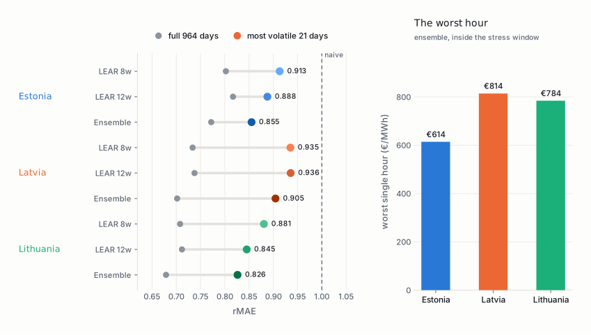
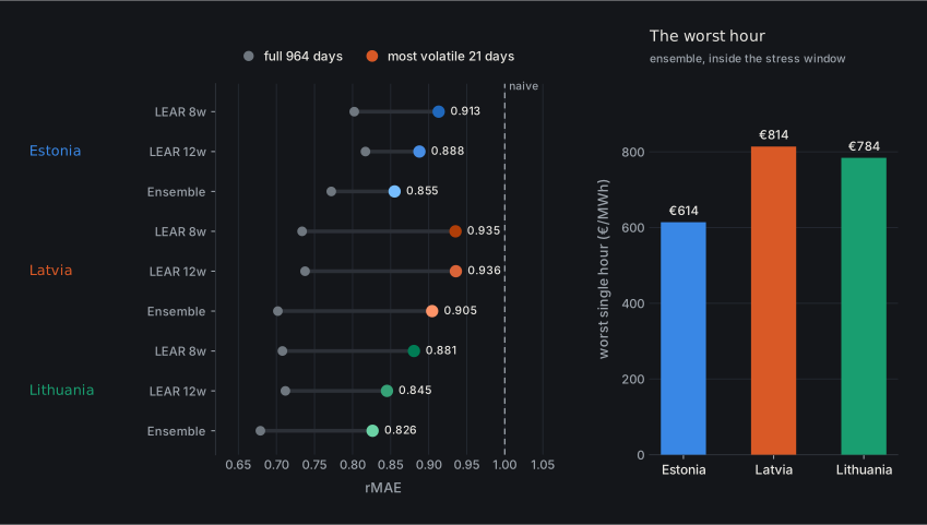
The Latvian result is the sharpest. Inside its most volatile 21 days, the ensemble keeps only a 9.5% MAE advantage over a forecast that copies last week — against 29.8% over the full sample. Two thirds of the model’s value evaporates precisely when it would be worth the most.
Large hourly errors define these episodes. The ensemble’s worst single hour reaches €614/MWh in Estonia, €814/MWh in Latvia and €784/MWh in Lithuania. Figure 11 shows where those misses sit: the model tracks the general level competently and then flattens against a spike that arrives without warning in its own information set.
Two further results are worth recording. First, the ensemble remains the best specification in every zone under stress, so forecast averaging buys robustness and not only average accuracy. Second, the ranking of the two individual windows flips: the 12-week model beats the 8-week model in Estonia and Lithuania inside their stress windows, and the two are indistinguishable in Latvia. The shortest available history is not automatically the best one when the price regime turns — more history can buy stability at exactly the moment adaptiveness stops helping.
5. Limitations and extensions
This is not a full replication. The original LEAR benchmark estimates 8-week, 12-week, three-year and four-year specifications and combines all four. Computational cost restricted this work to the two short windows, which is why the combination is called a short-window ensemble everywhere above and never just “the ensemble”.
The information set is deliberately thin. The model sees local price history, a load forecast and a wind forecast. The Baltic zones are among the most tightly interconnected in Europe, and the archive already holds scheduled exchanges, physical cross-border flows, transmission and generation outages, installed capacity, balancing data and neighbouring-system series. Whether market integration variables improve accuracy is the natural next question. It has to be asked carefully: realized flows or realized generation for the delivery hour must never enter contemporaneously, only information known before gate closure or properly lagged realized values.
Missing data required judgement. Short gaps were interpolated and one isolated Estonian wind-forecast day was reconstructed from its neighbours. The affected share of observations is small, but a production implementation should formalise the missing-data policy and test whether the choice of imputation moves the forecasts at all.
One implementation detail is load-bearing. The epftoolbox LEAR routine needed a compatibility adjustment to LassoLarsIC under modern Python/scikit-learn when the number of candidate predictors exceeds the number of observations — which is exactly the regime the short windows sit in. The adjustment preserves the LEAR framework, but it is the kind of thing that has to be documented for anyone reproducing the numbers.
There is no significance testing. Every comparison above is a comparison of point metrics. Lago et al. are explicit that predictive-accuracy differences need formal testing, and the multivariate Diebold–Mariano and Giacomini–White tests across the 8-week, 12-week, ensemble and naive forecasts are the single highest-value addition to this analysis.
The synchronisation analysis is descriptive. February 2025 is an operationally significant date, but comparing metrics either side of it identifies nothing causal. A stronger design would use change-point tests on prices and on forecast errors, rolling coefficient stability, and interactions with transmission and balancing conditions.
The stress windows were selected after the fact. They are a stress test, not an unbiased estimate of anything. The primary evidence remains the full 964-day evaluation. A more complete treatment would classify all days into volatility quantiles and compare accuracy across the whole distribution rather than the single most extreme interval.
Only one benchmark was run. Lago et al. identify the DNN as the stronger and more expensive benchmark, with LEAR attractive for its low complexity and fast recalibration. Running the DNN on the same Baltic datasets would establish whether nonlinearity buys anything economically meaningful over a strong linear baseline.
6. Conclusion
This project runs an electricity price forecasting workflow end to end: automated collection of a large European power-market database, construction of leakage-safe day-ahead inputs, implementation of a recognised benchmark model, rolling out-of-sample evaluation across three bidding zones, and explicit stress testing where the model is most likely to fail.
The central result is consistent across all three markets. LEAR substantially outperforms a weekly naive forecast, and averaging the 8-week and 12-week specifications improves on both. The short-window ensemble cuts MAE against the naive benchmark by roughly 23% in Estonia, 30% in Latvia and 32% in Lithuania.
The second result matters as much. Accuracy degrades sharply when prices turn volatile. Relative performance stays better than naive, but the margin narrows — to 9.5% in Latvia — and individual hourly errors run past €600–800/MWh. The central difficulty of electricity price forecasting is visible in the gap between those two paragraphs: a model can look strong on average while remaining exposed to exactly the observations that carry the commercial risk.
LEAR is a credible, cheap baseline for Baltic day-ahead prices. The ENTSO-E archive assembled here is the more valuable output — it is what makes the obvious next steps possible: cross-border information, outage and balancing variables, longer calibration windows, formal predictive-accuracy testing, and nonlinear benchmarks.
References
Lago, J., Marcjasz, G., De Schutter, B., & Weron, R. (2021). Forecasting day-ahead electricity prices: A review of state-of-the-art algorithms, best practices and an open-access benchmark. Applied Energy, 293, 116983. [Paper] [epftoolbox]
Uniejewski, B., Weron, R., & Ziel, F. (2018). Variance stabilizing transformations for electricity spot price forecasting. IEEE Transactions on Power Systems, 33(2), 2219–2229. [Paper]
Diebold, F. X., & Mariano, R. S. (1995). Comparing predictive accuracy. Journal of Business & Economic Statistics, 13(3), 253–263. [Paper]
ENTSO-E. Transparency Platform. [Data]