Systems Decision Lab

Studying petabyte-scale scientific workflows on a laptop, by simulating their metadata instead of their data.

The Einstein Telescope is expected to produce data workflows at the petabyte scale, with heterogeneous compute demands and scheduling problems that nobody has solved yet. Someone has to design the methods that will manage those workflows. The awkward part is that designing them appears to require the thing being designed for: continuous access to petabyte datasets and to the expensive machines that process them. Students and research teams do not have that access, so the methods tend to get built late, by whoever is already inside the facility, and tested once rather than compared.

This project is my attempt at the cheap layer that should come first. It represents a workflow as lightweight task metadata, simulates that metadata under constrained resources, and lets scheduling and capacity decisions be tested and compared on an ordinary laptop. It is not a replacement for experiments on real infrastructure. It is the thing you use before them, so that you arrive at the real machine with a short list instead of a blank page.

Simulating the description instead of the data

The move the whole project rests on is separating the logical scale of a workflow from its physical scale. A workflow might represent terabytes or petabytes of science, but if the question is when tasks run, what they wait for, and where queues form, then the contents of those bytes never enter the calculation. What matters is how long a task occupies which resources, and when it shows up. So the simulator keeps that and throws away everything else.

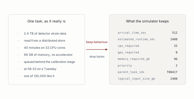
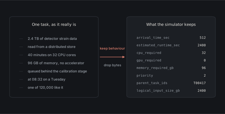
Figure 1. What survives the abstraction. The left column is a task as it exists; the right column is everything the simulator needs in order to reason about when it runs.

The practical consequence is a change of several orders of magnitude. A workload of 120,000 tasks representing a few petabytes of logical data is roughly 40 MB of CSV. It loads into memory on any laptop, and a simulated run of it finishes in seconds.

The limitation is in the same sentence as the benefit. This abstraction is only valid for questions where the content of the data does not matter. Ask about data movement, cache behaviour or network topology, and the thing you dropped is exactly the thing you needed. I come back to that below, because it is the honest boundary of the approach rather than a to-do item.

Why the clock jumps

The engine is a discrete-event simulator, and this is the part I would most want to defend, because it is what makes the rest affordable.

A time-stepped simulation advances a fixed interval at a time and recomputes the state of the system at each step. Most of that work is wasted. Between one task finishing and the next arriving, nothing about the system changes, so there is nothing to recompute. An event-driven engine instead keeps a queue of the moments when the state will change and jumps the clock straight to the next one.

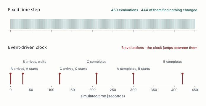
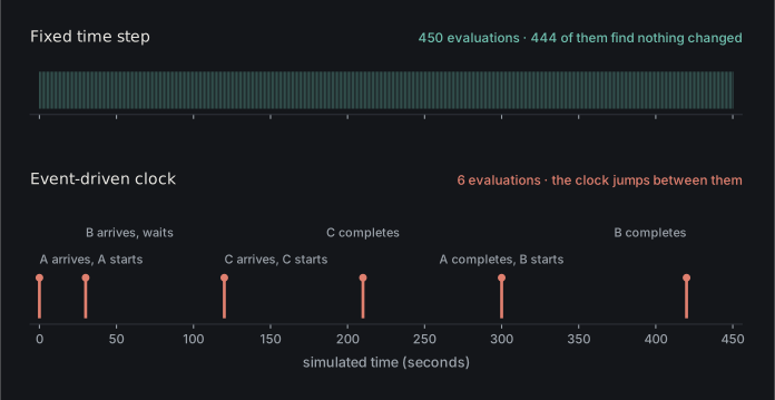
Figure 2. The same three-task scenario under both schemes. Stepping one second at a time takes 450 evaluations, 444 of which find nothing has changed. The event-driven clock touches six moments, which are the only six at which anything happens.

The important property is what the cost scales with. A time-stepped run costs more if you simulate a longer horizon or choose a finer resolution, even when the workload is identical. An event-driven run costs what the workload costs: one arrival event per task, one completion event per task that runs. A month-long workload of 50,000 tasks is about 100,000 events, whichever way you slice the calendar.

That is not just an efficiency note. It is what makes the experimental design possible. If a single run is cheap, you can afford to run the same workload under four scheduling policies, at a dozen seeds, across a sweep of cluster configurations, and talk about distributions of outcomes rather than one anecdote. An expensive simulator gets used once and quoted; a cheap one gets used properly.

How the engine is put together

Five components carry the entire simulation.

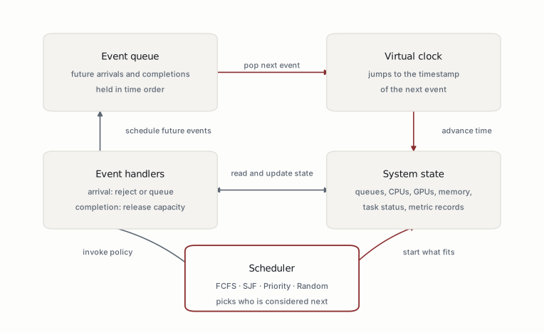
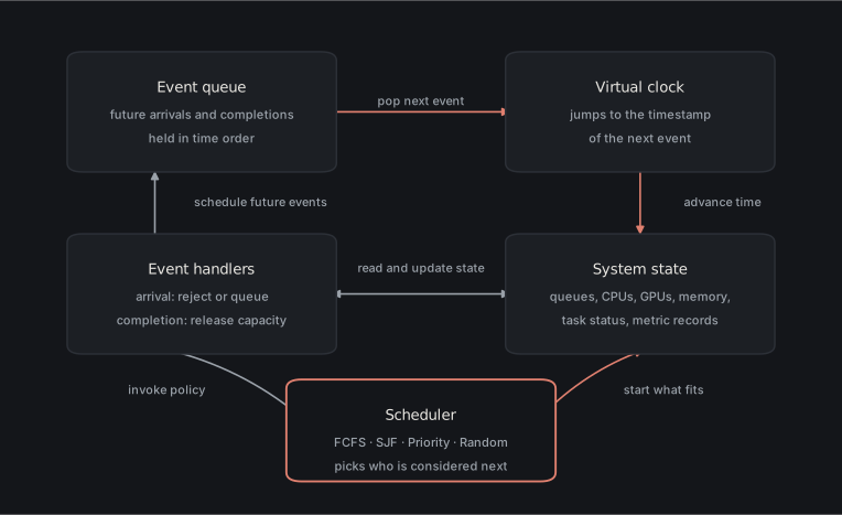
Figure 3. One turn of the loop. The queue holds the future, the clock jumps to it, a handler changes the state, and the scheduler decides who gets the capacity that just became available.

The event queue is the timeline. At the start it holds one arrival event per task, in time order; every time a task starts running, a completion event is pushed onto it at the appropriate future time. The virtual clock does no work of its own — it simply takes the timestamp of whatever event comes off the queue next. The system state is the simulated cluster: total and available CPUs, GPUs and memory, plus the waiting, running, completed and rejected tasks, updated after every event.

The handlers contain the logic. When a task arrives, the first question is not whether it can run now but whether it could ever run: if it asks for more CPUs, GPUs or memory than the whole cluster has, it is marked rejected rather than left in a queue forever. That case is reported in the output rather than hidden, because in practice it usually means the workload assumptions and the cluster configuration disagree, and it is better to be told that than to watch a queue never drain. Otherwise the task joins the waiting queue and the scheduler is invoked. When a task completes, its resources go back to the pool, its timings are recorded, and the scheduler is invoked again, because capacity has just appeared.

The scheduler is the part that is meant to be swapped. It orders the waiting queue according to a policy — first-come first-served, shortest job first, priority, random — and the engine then starts every task that fits, in that order. It is worth being explicit about one design decision here: a task the policy ranks first but that does not currently fit does not block the queue. The engine keeps looking, so a two-core job is not stuck behind a fourteen-core one waiting for a hole. That is a deliberate modelling choice resembling backfilling on a real batch system, and it materially changes the results, so it belongs in the description of the model rather than buried in the code.

What one run looks like

Here is an actual run: thirteen tasks against a cluster of 16 CPUs, 2 GPUs and 256 GB, under first-come first-served. The whole simulation is thirty-seven events.

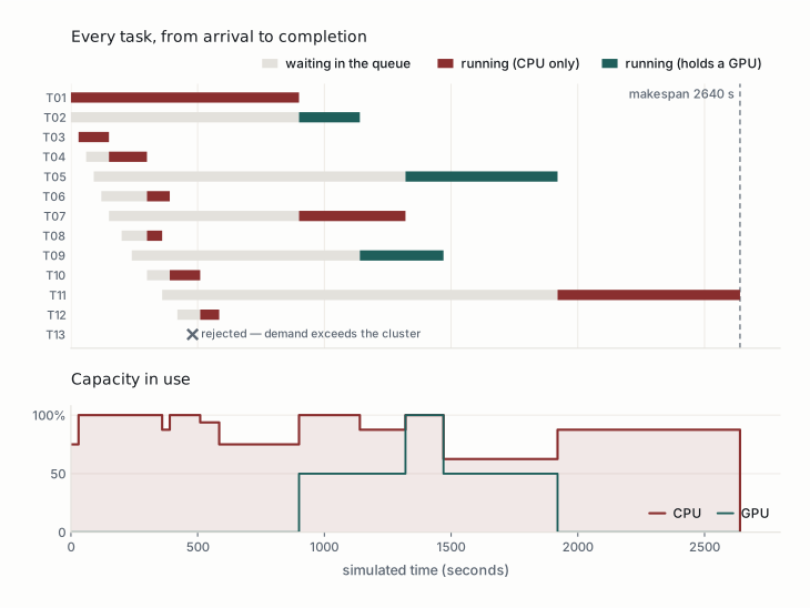
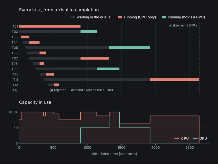
Figure 4. One simulated run. Each task waits (grey) and then runs (colour); the lower panel is the fraction of CPU and GPU capacity held at each moment. Nothing here was drawn by hand — it is the engine’s output for this workload.

The figure shows the kind of thing that is hard to reason about on paper. T01 takes twelve of the sixteen cores for the first 900 seconds, so for that whole period the cluster behaves as though it were a four-core machine, and only small tasks fit in the gap. T11 needs fourteen cores; it arrives at 360 seconds and does not start until 1920, having waited 1560 seconds for a hole large enough to hold it, while eight smaller tasks that arrived after it have come and gone. T13 asks for 24 cores on a 16-core cluster and is rejected at arrival. The GPU trace shows a resource that is either half idle or fully saturated and never anything in between, because only three tasks in this workload want one.

Each run produces a task-level table with the full lifecycle of every task, a queue timeline, a resource-utilization timeline, and the aggregate metrics you would expect: makespan, completion rate, mean and median wait, turnaround, throughput, mean utilization per resource, and total core-seconds. The queue timeline is where backlog formation shows up; the utilization timeline is where you find out whether you are CPU-bound, GPU-bound, memory-bound, or simply scheduling badly.

The comparison is the point

A single run is a description. The reason to build the thing is comparison, and comparison is only meaningful if it is controlled: hold the workload fixed, hold the cluster fixed, hold the seeds and runtime assumptions fixed, change one policy, and attribute the difference to that policy under those stated conditions.

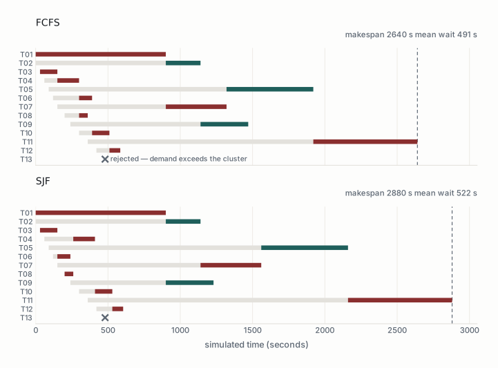
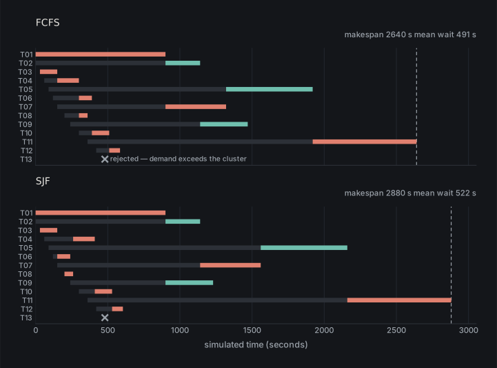
Figure 5. Identical workload, identical cluster, identical seed; only the scheduling policy differs. Shortest job first, the textbook choice for minimising waiting time, does worse here on both measures.

That result is the reason I find this worth doing. Shortest job first is supposed to minimise mean waiting time, and in the classical setting — one resource, all jobs present at the start — it does. Here it loses on both counts: mean wait rises from 491 to 522 seconds and makespan from 2640 to 2880. The mechanism is visible in the figure. Because the engine already lets small tasks slip into gaps, first-come first-served is not actually starving them; meanwhile shortest job first keeps deferring the two widest tasks, T05 and T11, until almost everything else has drained, and the run acquires a long thin tail where the cluster is mostly idle. Priority scheduling and random selection both land near 658 seconds of mean wait, worse than either.

I am not claiming first-come first-served is the better policy. The claim is narrower and more useful: with multiple resource dimensions, staggered arrivals and backfilling, the textbook ranking does not survive, and which policy wins depends on the shape of the workload rather than on the policy alone. That is precisely the kind of question you cannot settle by argument, and precisely why a cheap testbed earns its place.

The workload description turned out to be the hard part

The engine itself is a few hundred lines. Most of the code in the repository is not the simulator — it is the machinery for describing the workload, and that surprised me at first. The reason is that a simulation result is worth exactly as much as the workload description behind it, and a workload description is a scientific claim. If I tell you that a policy reduces mean wait by 12%, your next question should be where my runtime estimates came from, and whether you can reproduce the workload I ran them on. Without an answer, the number is decoration.

So the metadata layer is built to answer that. The canonical schema is 81 fields, and its most important property is that it refuses to mix different kinds of statement: what a task requested, what it was allocated, what was observed, its peak use, what was estimated from assumed rates, and what was actually billed are separate fields that stay null when unknown. A measurement never quietly becomes an assumption. Validation runs structural, temporal, semantic, provenance, referential and dependency checks, produces a weighted quality score, and can block a release outright — a scenario with an unassigned owner or missing provenance is not fit to base a decision on, however clean its numbers look.

Reproducibility is enforced rather than hoped for: the same configuration and seed produce byte-identical output, and a release is exported as a bundle carrying the configuration, validation report, per-artifact checksums, the runtime environment and a contract stating exactly what a third party needs in order to regenerate it. Real traces can be imported instead of generated — there are adapters for Slurm accounting records, Kubernetes, Airflow, Spark, Prometheus and others — with every canonical field traceable back to a source column, a documented default or an explicit rule, and automatic mappings always requiring review before they commit. Given a real trace, the system can also fit a synthetic twin and score how closely it matches on distributions, correlations, arrivals and tail coverage. That score is reported alongside a warning I think is important: fidelity is not validity. A twin can match a trace closely and still represent the wrong population.

What it cannot do

The engine does not model data movement, network contention, storage latency or distributed file systems. It does not talk to SLURM, Kubernetes or MPI. It does not model node failures or real detector pipelines. These are deliberate exclusions at this stage rather than an unwritten roadmap: they are what keeps the model small enough to explain and cheap enough to run.

Two limits matter more than that list. The first is that runtime is an input, not a prediction. Every result is conditional on runtime estimates being roughly right, and if they are systematically wrong the simulator will produce confident, internally consistent, wrong answers, with nothing in its output to indicate the problem. The second is that no simulator validates itself. Until this has been fitted to real scheduler logs and backtested against what those systems actually did, it is an instrument for generating hypotheses about scheduling, not evidence about any particular facility.

What I would want to do next

Four questions follow directly from the current state, and they are the ones I would want to work on.

The first is uncertainty. Every result above treats runtime as a point estimate, when real runtimes are distributions with heavy tails. Propagating that properly means asking whether the ranking between policies is stable under runtime uncertainty or whether it flips, and the answer determines how much any comparison of this kind is worth.

The second is learned policies. The natural use of a cheap simulator is to train a scheduling policy in it, which immediately raises the sim-to-real question: does a policy trained on metadata transfer to a real batch system, and can the size of the transfer gap be predicted from the fidelity score of the workload it was trained on? That is the question I find most interesting, because it makes the fidelity machinery do real work rather than sit in a report.

The third is validation, which is the precondition for the other two: fit real HPC scheduler logs, backtest the simulator against recorded outcomes, and publish the gap honestly.

The fourth is the boundary of the abstraction itself. Adding data movement and network constraints and then measuring how much the conclusions move would answer whether metadata-only simulation is sufficient, and for which class of question. If the answers barely change, the abstraction is justified; if they change a lot, that is a more interesting result and worth knowing early.

Where it came from

The project began as a research proposal for ETCETERA, the programme preparing the Einstein Telescope for the era of gravitational-wave astronomy, titled Simulating Petabyte-Scale Scientific Workflows Without Petabyte Data. Gravitational-wave computing is the motivating case, but nothing in the kernel is specific to it: tasks, events, resources, policies and evidence are domain-neutral, and the domain vocabulary lives in labels, adapters and extension fields. The same machinery applies to data centres, industrial workflows and other scientific facilities.

Status

Active research build. The metadata, validation, calibration and governance layers are usable end to end; the event-driven engine currently runs as a separate prototype and is being folded into the same pipeline. Interfaces will still change.

• Source
• Run it locally: pip install -r requirements.txt, then python -m streamlit run app.py
• The engine used for Figures 2, 4 and 5 on this page is _engine.py in this folder; _figures.py rebuilds every figure from its output.